Most communication systems (human speech, sonar, microwave, radio, co-ax, fiber optics, twisted pair etc) are simply described in terms of:
- Transmitter power
- Transmission path degradation
- Receiver sensitivity (power)
It is therefore quite natural that communications engineers should use a system of units and measurements that enables these three elements to be easily defined and calculated.
Note that transmitter power and receiver sensitivity are absolute power levels (e.g. Watts or dBm), whereas the transmission path degradation is a relative value (e.g. % signal reduction or dB), which is generally independent of the actual power level involved. Path degradation may involve a combination of factors, such as attenuation and dispersion. No-attenuation factors such as dispersion are often summarized as a simple "equivalent loss" penalty, so they can be treated in the same way,
The universal measurement system adopted for this purpose is the Decibel, which is a logarithmic unit. The decibel unit allows these 3 system parameters to be easily calculated by addition and subtraction, rather than multiplication and division.
Example
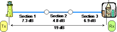
How this makes calculations simple is shown in an example of a fiber optic transmission system:
Absolute power levels in this example are expressed in dBm and generally refer to input and output power levels. The 'm' refers to the reference level used, in this case mW (milli Watts).
The reference level for optical systems is usually 1 mW, since the absolute transmitter power is often about this power level, making it a convenient stating point. A value of 0 dBm is 1 mW.
Let's look at the allowable loss budget for a typical system, typically taken the equipment data sheet:
| Emitter power |
-4 dBm |
| Receiver sensitivity |
-27 dBm |
Allowable degradation, or loss budget: -4 -27 = 23 dB.
Note that "loss" really means "negative" so a loss of 23 dB means -23 dB allowable loss.
(A negative loss would be a gain)
Signal attenuation in this example is defined in dB units and generally refers to transmission path losses (Lossy transmission path)
Let's look at the measured loss of 3 actual fiber lengths joined up:
| Signal decrease of 1st fiber section |
7.3 dB |
| Signal decrease of 2nd section |
4.8 dB |
| Signal decrease of 3rd section |
6.9 dB |
So the measured transmission degradation of the complete link is 7.3 + 4.8 + 6.9 = 19 dB
| Therefore, spare system margin |
-19 - (-23) = 4 dB? |
In this example system, if the measured transmission loss is 19 dB, then you'd think that the spare system margin is 4 dB.
However, some allowance must be made for measuring uncertainties. Suppose the power and loss test accuracy is plus or minus 0.41 dB (e.g. 10%) for each of the 2 absolute power measurements, and each of the 3 loss measurements, then that's 5 lots of 0.41 dB uncertainty, This is where the maths gets a bit difficult, since dB uncertainties do not just add and, and in any case linear uncertainties are most easily added using an rms method.
Here is a summary of wrong and right maths results:
- Wrong! Uncertainty = 5 x 0.41 dB = 2.05 dB
- Wrong! Uncertainty = "rms of 5 x .41 dB" = 0.92 dB (not very far off)
- Wrong! Uncertainty = 5 x 10 % = 50 % = 1.76 dB
- Right! Uncertainty = "rms of 5 x 10 %" = 22.4 % = 0.88 dB
So in this case, the system margin can be stated as 4 - 0.88 = 3.12 dB with 95% confidence
You can see here how test uncertianty can eat into precious system margin!
Note there are a few ways to "correctly" calculate uncertainty. The most recent one is the Welch-Satterthwaite equation; however this is more complex and beyond this article. It is used in calibration laboratories and may result in slightly smaller uncertainty values. The traditional RMS method shown here is more readily understood and is quite adequate for most purposes.
So test accuracy is important to reduce measurement uncertainty. Improved test accuracy results directly in allowing more variability in acceptance criteria. For example, an allowable measured margin of 3.12 dB in the above case might not be acceptable, resulting in increased rework.
The definition of the dBm unit is:
dB = 10 log10 (P1⁄P2)
where...
P1 = Measured power level (e.g in Watts)
P2 = Reference power level (e.g in Watts)
P2 is fixed (typically at 1 milliwatt) for dBm
If P2 is not fixed, this is also known as the 'decibel (or dB) definition'.
A simple dBm/dB calculator:
Some sample values:
| dBm Power unit |
mW power unit |
dBm Power unit |
mW power unit |
| +20 |
100 mW |
-30 |
1 µW |
| +10 |
10 mW |
-40 |
100 nW |
| 0 |
1 mW |
-50 |
10 nW |
| -10 |
100 µW |
-60 |
1 nW |
| -20 |
10 µW |
-70 |
100 pW |
For relative dB measurements, P2 is arbitrarily defined by the user:
| dB |
Relative value |
|
dB |
Relative value |
| +20 |
x100 |
102 |
|
-30 |
/1,000 |
10-3 |
| +10 |
x 10 |
101 |
|
-40 |
/10,000 |
10-4 |
| 0 |
x 1 |
100 |
|
-50 |
/100,000 |
10-5 |
| -10 |
/10 |
10-1 |
|
-60 |
/1 million |
10-6 |
| -20 |
/100 |
10-2 |
|
-70 |
/10 million |
10-7 |
The dBm decibels unit also has the following useful attributes:
- It reduces large numbers to a convenient size (e.g. -70 dB = 1/10,000,000).
- It offers constant resolution for a given number of decimal places, which improves calculation confidence. 0.1 dB gives 2.3 % resolution. 0.01 dB gives 0.23 % resolution.
- It is a universal unit that an engineer can apply to any communications link.
How much dBm / dB measurement resolution do I need?
Meters are available with resolution ranging from 0.1 to 0.001 dB / dBm, with cost differences to match:
0.001 dBm / dB (0.023%) resolution may be occasionally useful in carefully controlled laboratory conditions, with an expert user. Absolute optical power standards are now accruate to about 0.2%.
0.1 dB (2.3%) resolution may not be enough. This performance is often adequate to measure absolute power levels but cannot measure connector or splice loss with sufficient precision, since the measurement uncertainty involved is larger than the expected test value. Uncertainty must be in excess of ± 0.14 dB (e.g. ± 1 digit, over 2 measurements).
0.01 dB (0.23%) resolution is ideal for most work on fibre systems. It is for this reason that Kingfisher instruments generally provide a resolution of 0.01 dB.
Calculating dBm measurement uncertainty
To calculate the total measurement uncertainty, the following rules are handy:
Linear uncertainty can be added using the RMS method. For example the total of 3 uncertainties of 4 %, 3 % and 2 %, = √(42 + 32 + 22 ) = 5.4 % (not 9 %).
However dBm / dB uncertainty values must be converted to linear values and then averaged using the above method.
In practice, this inconvenience can often be avoided by use of a "decibel math" rule of thumb as follows:
If the 2nd highest logarithmic value is less than 80% of the highest value, the uncertainty is approximated to the largest value.
If the 2nd highest value is over 80% of the highest value, multiply the highest value by 1.4 for the combined figure.
In practical situations, one or two uncertainty figures tend to dominate the others. Here are some examples:
Three different uncertainty values of 0.3 dB, 0.2 dB, 0.1 dB, give a combined uncertainty of 0.35 dB. The error in ignoring the lower values is only 0.05 dB.
Two similar uncertainty values of 0.3 and 0.29 dB, give a combined uncertainty of 0.39 dB. The approximated figure is 0.42 dB, out by only 0.03 dB.
Five different uncertainty values of 0.4, 0.2, 0.1, ,0.09, 0.05 dB give a combined uncertainty of 0.42 dB. This is within 0.02 dB of the approximated figure of 0.4 dB.
dB averaging
Within the telecommunications industry, link attenuation is commonly calculated by averaging a bi-directional measurement. There are various reasons given for this, but the most important practical reasons are that this method eliminates meter calibration errors and minimizes the effects of source drift. This is of course simple stuff; however the hidden flaw is that it is mathematically incorrect for logarithmic or dB units to be treated this way. The correct method is to first convert to linear, then average and finally convert back to dB. Further reading on this topic can be found in Kingfisher Application Note A14, Improving Attenuation Measurement Accuracy
Electro-optic conversion:
Optical signals are usually converted to an electric current, which is then measured as a voltage across a resistor (in a trans-impedance amplifier).
The electrical power dissipated by the resistor goes up with the square of the voltage.
So the optical receiver power also goes up with the square of the optical signal.
So when working in volts, the relationship is defined as: dB = 20 log (V1/V2)
Where
V1 = measured voltage
V2 = reference voltage (e.g. 1 mV)
More information